Difference between revisions of "त्रिकोणमितीय पहचान की सूची"

Revision as of 11:05, 6 July 2022

Template:Trigonometry त्रिकोणमिति में, त्रिकोणमितीय पहचान समानताएं होती हैं जो त्रिकोणमितीय कार्यों को शामिल करती हैं और घटित चर के प्रत्येक मूल्य के लिए सही होती हैं, जिसके लिए समानता के दोनों पक्षों को परिभाषित किया जाता है।ज्यामितीय रूप से, ये एक या एक से अधिक कोणों के कुछ कार्यों से जुड़ी पहचान हैं।वे त्रिभुज पहचान से अलग हैं, जो संभावित रूप से कोणों को शामिल करने वाली पहचान हैं, लेकिन एक त्रिभुज की लंबाई या अन्य लंबाई भी शामिल हैं।

जब भी त्रिकोणमितीय कार्यों से जुड़े अभिव्यक्तियों को सरल बनाने की आवश्यकता होती है, तो ये पहचान उपयोगी होती हैं।एक महत्वपूर्ण एप्लिकेशन गैर-सैन्य-संबंधी कार्यों का एकीकरण है: एक सामान्य तकनीक में पहले एक त्रिकोणमितीय फ़ंक्शन के साथ प्रतिस्थापन नियम का उपयोग करना शामिल होता है, और फिर एक त्रिकोणमितीय पहचान के साथ परिणामी अभिन्न को सरल बनाता है।

पाइथागोरियन पहचान

साइन और कोसाइन के बीच मूल संबंध पाइथागोरियन पहचान द्वारा दिया गया है:

\sin ^{2}\theta +\cos ^{2}\theta =1,

कहाँ पे $\sin ^{2}\theta$ साधन $(\sin \theta )^{2}$ तथा $\cos ^{2}\theta$ साधन $(\cos \theta )^{2}.$ इसे पाइथागोरियन प्रमेय के एक संस्करण के रूप में देखा जा सकता है, और समीकरण से अनुसरण करता है $x^{2}+y^{2}=1$ यूनिट सर्कल के लिए।इस समीकरण को साइन या कोसाइन के लिए हल किया जा सकता है:

{\begin{aligned}\sin \theta &=\pm {\sqrt {1-\cos ^{2}\theta }},\\\cos \theta &=\pm {\sqrt {1-\sin ^{2}\theta }}.\end{aligned}}

जहां संकेत के चतुर्थांश पर निर्भर करता है $\theta .$ इस पहचान को विभाजित करना $\sin ^{2}\theta$ , $\cos ^{2}\theta$ , या दोनों निम्नलिखित पहचान प्राप्त करते हैं:

1+\cot ^{2}\theta =\csc ^{2}\theta

\tan ^{2}\theta +1=\sec ^{2}\theta

\sec ^{2}\theta +\csc ^{2}\theta =\sec ^{2}\theta \csc ^{2}\theta

इन पहचानों का उपयोग करते हुए, किसी भी अन्य (प्लस या माइनस साइन तक) के संदर्भ में किसी भी त्रिकोणमितीय फ़ंक्शन को व्यक्त करना संभव है:

Each trigonometric function in terms of each of the other five.^[1]
in terms of	$\sin \theta$	$\csc \theta$	$\cos \theta$	$\sec \theta$	$\tan \theta$	$\cot \theta$
$\sin \theta =$	$\sin \theta$	${\frac {1}{\csc \theta }}$	$\pm {\sqrt {1-\cos ^{2}\theta }}$	$\pm {\frac {\sqrt {\sec ^{2}\theta -1}}{\sec \theta }}$	$\pm {\frac {\tan \theta }{\sqrt {1+\tan ^{2}\theta }}}$	$\pm {\frac {1}{\sqrt {1+\cot ^{2}\theta }}}$
$\csc \theta =$	${\frac {1}{\sin \theta }}$	$\csc \theta$	$\pm {\frac {1}{\sqrt {1-\cos ^{2}\theta }}}$	$\pm {\frac {\sec \theta }{\sqrt {\sec ^{2}\theta -1}}}$	$\pm {\frac {\sqrt {1+\tan ^{2}\theta }}{\tan \theta }}$	$\pm {\sqrt {1+\cot ^{2}\theta }}$
$\cos \theta =$	$\pm {\sqrt {1-\sin ^{2}\theta }}$	$\pm {\frac {\sqrt {\csc ^{2}\theta -1}}{\csc \theta }}$	$\cos \theta$	${\frac {1}{\sec \theta }}$	$\pm {\frac {1}{\sqrt {1+\tan ^{2}\theta }}}$	$\pm {\frac {\cot \theta }{\sqrt {1+\cot ^{2}\theta }}}$
$\sec \theta =$	$\pm {\frac {1}{\sqrt {1-\sin ^{2}\theta }}}$	$\pm {\frac {\csc \theta }{\sqrt {\csc ^{2}\theta -1}}}$	${\frac {1}{\cos \theta }}$	$\sec \theta$	$\pm {\sqrt {1+\tan ^{2}\theta }}$	$\pm {\frac {\sqrt {1+\cot ^{2}\theta }}{\cot \theta }}$
$\tan \theta =$	$\pm {\frac {\sin \theta }{\sqrt {1-\sin ^{2}\theta }}}$	$\pm {\frac {1}{\sqrt {\csc ^{2}\theta -1}}}$	$\pm {\frac {\sqrt {1-\cos ^{2}\theta }}{\cos \theta }}$	$\pm {\sqrt {\sec ^{2}\theta -1}}$	$\tan \theta$	${\frac {1}{\cot \theta }}$
$\cot \theta =$	$\pm {\frac {\sqrt {1-\sin ^{2}\theta }}{\sin \theta }}$	$\pm {\sqrt {\csc ^{2}\theta -1}}$	$\pm {\frac {\cos \theta }{\sqrt {1-\cos ^{2}\theta }}}$	$\pm {\frac {1}{\sqrt {\sec ^{2}\theta -1}}}$	${\frac {1}{\tan \theta }}$	$\cot \theta$

प्रतिबिंब, बदलाव, और आवधिकता

यूनिट सर्कल की जांच करके, कोई त्रिकोणमितीय कार्यों के निम्नलिखित गुणों को स्थापित कर सकता है।

↑ Abramowitz and Stegun, p. 73, 4.3.45

[1] Abramowitz and Stegun, p. 73, 4.3.45

[1]

Difference between revisions of "त्रिकोणमितीय पहचान की सूची"

Revision as of 11:05, 6 July 2022

पाइथागोरियन पहचान

प्रतिबिंब, बदलाव, और आवधिकता

Navigation menu

Search

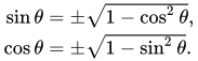
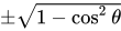
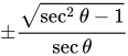
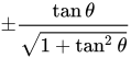
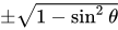
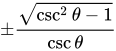
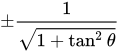
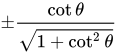
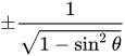
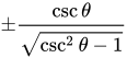
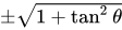
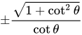
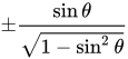
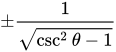
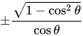
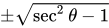
@@ Line 87: / Line 87: @@
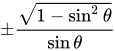
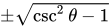
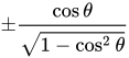
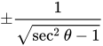
 यूनिट सर्कल की जांच करके, कोई त्रिकोणमितीय कार्यों के निम्नलिखित गुणों को स्थापित कर सकता है।
-=== प्रतिबिंब ===
+[[Category:Pages with broken file links]]
-जब एक यूक्लिडियन वेक्टर की दिशा को एक कोण द्वारा दर्शाया जाता है <math>\theta,</math> यह मुक्त वेक्टर (मूल में शुरू) और सकारात्मक द्वारा निर्धारित कोण है <math>x</math>-इकाई वेक्टर।एक ही अवधारणा को एक यूक्लिडियन स्थान में लाइनों पर भी लागू किया जा सकता है, जहां कोण यह है कि मूल और सकारात्मक के माध्यम से दी गई रेखा के समानांतर द्वारा निर्धारित किया जाता है <math>x</math>-एक्सिस।यदि दिशा के साथ एक लाइन (वेक्टर) <math>\theta</math> दिशा के साथ एक रेखा के बारे में परिलक्षित होता है <math>\alpha,</math> फिर दिशा कोण <math>\theta^{\prime}</math> इस परावर्तित लाइन (वेक्टर) का मान है
-<math display="block">\theta^{\prime} = 2 \alpha - \theta.</math>
-इन कोणों के त्रिकोणमितीय कार्यों के मान <math>\theta,\;\theta^{\prime}</math> विशिष्ट कोणों के लिए <math>\alpha</math> सरल पहचान को संतुष्ट करें: या तो वे समान हैं, या विपरीत संकेत हैं, या पूरक त्रिकोणमितीय फ़ंक्शन को नियोजित करते हैं।इन्हें भी जाना जाता है {{em|reduction formulae}}.<ref>{{harvnb|Selby|1970|loc=p. 188}}</ref>
-| class = wikitable style = पृष्ठभूमि-रंग: #ffffff
-तू <math>\theta</math> झलक देना <math>\alpha = 0</math><ref>Abramowitz and Stegun, p.&nbsp;72, 4.3.13–15</ref><br/> <span style = font-weight: सामान्य> विषम/यहाँ तक कि पहचान </span>
-तू <math>\theta</math> झलक देना <math>\alpha = \frac{\pi}{4}</math>
-तू <math>\theta</math> झलक देना <math>\alpha = \frac{\pi}{2}</math>
-तू <math>\theta</math> झलक देना <math>\alpha = \frac{3\pi}{4}</math>
-तू <math>\theta</math> झलक देना <math>\alpha = \pi</math><br/> <स्पैन स्टाइल = फ़ॉन्ट-वेट: नॉर्मल> तुलना करें <math>\alpha = 0</math></span>
----
-|<math>\sin(-\theta) = -\sin \theta</math>
-|<math>\sin\left(\tfrac{\pi}{2} - \theta\right) =\cos \theta</math>
-|<math>\sin(\pi - \theta) = +\sin \theta</math>
-|<math>\sin\left(\tfrac{3\pi}{2} - \theta\right) =-\cos \theta</math>
-|<math>\sin(2\pi - \theta) = -\sin(\theta) = \sin(-\theta)</math>
----
-|<math>\cos(-\theta) =+ \cos \theta</math>
-|<math>\cos\left(\tfrac{\pi}{2} - \theta\right) = \sin \theta</math>
-|<math>\cos(\pi - \theta) = -\cos \theta</math>
-|<math>\cos\left(\tfrac{3\pi}{2} - \theta\right) = -\sin \theta</math>
-|<math>\cos(2\pi - \theta) = +\cos(\theta) = \cos(-\theta)</math>
----
-|<math>\tan(-\theta) = -\tan \theta</math>
-|<math>\tan\left(\tfrac{\pi}{2} - \theta\right) = \cot \theta</math>
-|<math>\tan(\pi - \theta) = -\tan \theta</math>
-|<math>\tan\left(\tfrac{3\pi}{2} - \theta\right) = +\cot \theta</math>
-|<math>\tan(2\pi - \theta) = -\tan(\theta) = \tan(-\theta)</math>
----
-|<math>\csc(-\theta) = -\csc \theta</math>
-|<math>\csc\left(\tfrac{\pi}{2} - \theta\right) = \sec \theta</math>
-|<math>\csc(\pi - \theta) =+ \csc \theta</math>
-|<math>\csc\left(\tfrac{3\pi}{2} - \theta\right) = -\sec \theta</math>
-|<math>\csc(2\pi - \theta) = -\csc(\theta) = \csc(-\theta)</math>
----
-|<math>\sec(-\theta) = +\sec \theta</math>
-|<math>\sec\left(\tfrac{\pi}{2} - \theta\right) = \csc \theta</math>
-|<math>\sec(\pi - \theta) = -\sec \theta</math>
-|<math>\sec\left(\tfrac{3\pi}{2} - \theta\right) = -\csc \theta</math>
-|<math>\sec(2\pi - \theta) = +\sec(\theta) = \sec(-\theta)</math>
----
-|<math>\cot(-\theta) = -\cot \theta</math>
-|<math>\cot\left(\tfrac{\pi}{2} - \theta\right) = \tan \theta</math>
-|<math>\cot(\pi - \theta) = -\cot \theta</math>
-|<math>\cot\left(\tfrac{3\pi}{2} - \theta\right) = +\tan \theta</math>
-|<math>\cot(2\pi - \theta) = -\cot(\theta) = \cot(-\theta)</math>
-|}
-=== शिफ्ट और आवधिकता ===
-[[File:Unit Circle - shifts.svg|thumb|right|upright=1.5|alt=Unit circle with a swept angle theta plotted at coordinates ए, बी)।चूंकि स्वेप्ट एंगल को एक-आधा पीआई (90 डिग्री) द्वारा बढ़ाया जाता है, इसलिए निर्देशांक को (-b, ए) में बदल दिया जाता है।एक-आधा पीआई (180 डिग्री कुल) की एक और वृद्धि निर्देशांक को (-a, -b) में बदल देती है।एक-आधा पीआई (270 डिग्री कुल) की एक अंतिम वृद्धि निर्देशांक को (बी, ए) में बदल देती है।> \ frac {\ pi} {2} </math>।]]
-{|class="wikitable" style="background-color: #FFFFFF"
-!Shift by one quarter period
-!Shift by one half period
-!Shift by full periods<ref>Abramowitz and Stegun, p.&nbsp;72, 4.3.7–9</ref>
-!Period
-|-
-|<math>\sin(\theta \pm \tfrac{\pi}{2}) = \pm\cos \theta</math>
-|<math>\sin(\theta + \pi) = -\sin \theta</math>
-|<math>\sin(\theta + k\cdot 2\pi) = +\sin \theta</math>
-|style="text-align: center;"|<math>2\pi</math>
-|-
-|<math>\cos(\theta \pm \tfrac{\pi}{2}) = \mp\sin \theta</math>
-|<math>\cos(\theta + \pi) = -\cos \theta</math>
-|<math>\cos(\theta + k\cdot 2\pi) = +\cos \theta</math>
-|style="text-align: center;"|<math>2\pi</math>
-|-
-|<math>\csc(\theta \pm \tfrac{\pi}{2}) = \pm\sec \theta</math>
-|<math>\csc(\theta + \pi) = -\csc \theta</math>
-|<math>\csc(\theta + k\cdot 2\pi) = +\csc \theta</math>
-|style="text-align: center;"|<math>2\pi</math>
-|-
-|<math>\sec(\theta \pm \tfrac{\pi}{2}) = \mp\csc \theta</math>
-|<math>\sec(\theta + \pi) = -\sec \theta</math>
-|<math>\sec(\theta + k\cdot 2\pi) = +\sec \theta</math>
-|style="text-align: center;"|<math>2\pi</math>
-|-
-|<math>\tan(\theta \pm \tfrac{\pi}{4}) =  \tfrac{\tan \theta \pm 1}{1\mp \tan \theta}</math>
-|<math>\tan(\theta + \tfrac{\pi}{2}) = -\cot \theta</math>
-|<math>\tan(\theta + k\cdot \pi) = +\tan \theta</math>
-|style="text-align: center;"|<math>\pi</math>
-|-
-|<math>\cot(\theta \pm \tfrac{\pi}{4}) =  \tfrac{\cot \theta \mp 1}{1\pm \cot \theta}</math>
-|<math>\cot(\theta + \tfrac{\pi}{2}) = -\tan\theta</math>
-|<math>\cot(\theta + k\cdot \pi) = +\cot \theta</math>
-|style="text-align: center;"|<math>\pi</math>
-|}
-== कोण योग और अंतर पहचान ==
-{{see also|Proofs of trigonometric identities#Angle sum identities|Small-angle approximation#Angle sum and difference}}
-[[File:AngleAdditionDiagramSine.svg|right|thumb|225px|तीव्र कोणों के साइन और कोसाइन के लिए कोण जोड़ के सूत्र का चित्रण।जोर दिया खंड इकाई लंबाई का है।]]
-इन्हें भी के रूप में जाना जाता है {{em|angle addition and subtraction theorems}} (या {{em|formulae}})।
-:<math>\begin{align}
-\sin(\alpha + \beta) &= \sin \alpha \cos \beta + \cos \alpha \sin \beta \\
-\sin(\alpha - \beta) &= \sin \alpha \cos \beta - \cos \alpha \sin \beta \\
-\cos(\alpha + \beta) &= \cos \alpha \cos \beta - \sin \alpha \sin \beta \\
-\cos(\alpha - \beta) &= \cos \alpha \cos \beta + \sin \alpha \sin \beta
-\end{align}</math>
-इन पहचानों को निम्नलिखित तालिका की पहले दो पंक्तियों में संक्षेपित किया गया है, जिसमें अन्य त्रिकोणमितीय कार्यों के लिए योग और अंतर पहचान भी शामिल हैं।
-{|class="wikitable" style="background-color:#FFFFFF"
-! Sine
-| colspan="3" style='border-style: solid none solid solid; text-align: right;' |<math>\sin(\alpha \pm \beta)</math>
-| style='border-style: solid none solid none; text-align: center;' |<math>=</math>
-| style='border-style: solid solid solid none; text-align: left;' |<math>\sin \alpha \cos \beta \pm \cos \alpha \sin \beta</math><ref>Abramowitz and Stegun, p.&nbsp;72, 4.3.16</ref><ref name="mathworld_addition">{{MathWorld|title=Trigonometric Addition Formulas|urlname=TrigonometricAdditionFormulas}}</ref>
-|-
-! Cosine
-| colspan="3" style='border-style: solid none solid solid; text-align: right;' |<math>\cos(\alpha \pm \beta)</math>
-| style='border-style: solid none solid none; text-align: center;' |<math>=</math>
-| style='border-style: solid solid solid none; text-align: left;' |<math>\cos \alpha \cos \beta \mp \sin \alpha \sin \beta</math><ref name="mathworld_addition"/><ref>Abramowitz and Stegun, p.&nbsp;72, 4.3.17</ref>
-|-
-! Tangent
-| colspan="3" style='border-style: solid none solid solid; text-align: right;' |<math>\tan(\alpha \pm \beta)</math>
-| style='border-style: solid none solid none; text-align: center;' |<math>=</math>
-| style='border-style: solid solid solid none; text-align: left;' |<math>\frac{\tan \alpha \pm \tan \beta}{1 \mp \tan \alpha \tan \beta}</math><ref name="mathworld_addition"/><ref>Abramowitz and Stegun, p.&nbsp;72, 4.3.18</ref>
-|-
-!Cosecant
-| colspan="3" style='border-style: solid none solid solid; text-align: right;' |<math>\csc(\alpha \pm \beta)</math>
-| style='border-style: solid none solid none; text-align: center;' |<math>=</math>
-| style='border-style: solid solid solid none; text-align: left;' |<math>\frac{\sec \alpha \sec \beta \csc \alpha \csc \beta}{\sec \alpha \csc \beta \pm \csc \alpha \sec \beta}</math><ref name=":0">{{Cite web|url=http://www.milefoot.com/math/trig/22anglesumidentities.htm|title=Angle Sum and Difference Identities|website=www.milefoot.com|access-date=2019-10-12}}</ref>
-|-
-! Secant
-| colspan="3" style='border-style: solid none solid solid; text-align: right;' |<math>\sec(\alpha \pm \beta)</math>
-| style='border-style: solid none solid none; text-align: center;' |<math>=</math>
-| style='border-style: solid solid solid none; text-align: left;' |<math>\frac{\sec \alpha \sec \beta \csc \alpha \csc \beta}{\csc \alpha \csc \beta \mp \sec \alpha \sec \beta}</math><ref name=":0" />
-|-
-! Cotangent
-| colspan="3" style='border-style: solid none solid solid; text-align: right;' |<math>\cot(\alpha \pm \beta)</math>
-| style='border-style: solid none solid none; text-align: center;' |<math>=</math>
-| style='border-style: solid solid solid none; text-align: left;' |<math>\frac{\cot \alpha \cot \beta \mp 1}{\cot \beta \pm \cot \alpha}</math><ref name="mathworld_addition"/><ref>Abramowitz and Stegun, p.&nbsp;72, 4.3.19</ref>
-|-
-! Arcsine
-| colspan="3" style='border-style: solid none solid solid; text-align: right;' |<math>\arcsin x \pm \arcsin y</math>
-| style='border-style: solid none solid none; text-align: center;' |<math>=</math>
-| style='border-style: solid solid solid none; text-align: left;' |<math>\arcsin\left(x\sqrt{1-y^2} \pm y\sqrt{1-x^2}\right)</math><ref>Abramowitz and Stegun, p.&nbsp;80, 4.4.32</ref>
-|-
-! Arccosine
-| colspan="3" style='border-style: solid none solid solid; text-align: right;' |<math>\arccos x \pm \arccos y</math>
-| style='border-style: solid none solid none; text-align: center;' |<math>=</math>
-| style='border-style: solid solid solid none; text-align: left;' |<math>\arccos\left(xy \mp \sqrt{\left(1-x^2\right)\left(1-y^2\right)}\right)</math><ref>Abramowitz and Stegun, p.&nbsp;80, 4.4.33</ref>
-|-
-! Arctangent
-| colspan="3" style='border-style: solid none solid solid; text-align: right;' |<math>\arctan x \pm \arctan y</math>
-| style='border-style: solid none solid none; text-align: center;' |<math>=</math>
-| style='border-style: solid solid solid none; text-align: left;' |<math>\arctan\left(\frac{x \pm y}{1 \mp xy}\right)</math><ref>Abramowitz and Stegun, p.&nbsp;80, 4.4.34</ref>
-|-
-! Arccotangent
-| colspan="3" style='border-style: solid none solid solid; text-align: right;' |<math>\arccot x \pm \arccot y</math>
-| style='border-style: solid none solid none; text-align: center;' |<math>=</math>
-| style='border-style: solid solid solid none; text-align: left;' |<math>\arccot\left(\frac{xy \mp 1}{y \pm x}\right)</math>
-|}
-=== सिन और अनंततापूर्ण रूप से कई कोणों के योगों के कोसाइन ===
-जब श्रृंखला <math display="inline">\sum_{i=1}^\infty \theta_i</math> तब बिल्कुल परिवर्तित होता है
-:<math>\sin\left(\sum_{i=1}^\infty \theta_i\right)
-=\sum_{\text{odd}\ k \ge 1} (-1)^\frac{k-1}{2}
-\sum_{\begin{smallmatrix} A \subseteq \{\,1,2,3,\dots\,\} \\ \left|A\right| = k\end{smallmatrix}}
-\left(\prod_{i \in A} \sin\theta_i \prod_{i \not \in A} \cos\theta_i\right)</math>
-:<math>\cos\left(\sum_{i=1}^\infty \theta_i\right)
-=\sum_{\text{even}\ k \ge 0} ~ (-1)^\frac{k}{2} ~~
-\sum_{\begin{smallmatrix} A \subseteq \{\,1,2,3,\dots\,\} \\ \left|A\right| = k\end{smallmatrix}}
-\left(\prod_{i \in A} \sin\theta_i \prod_{i \not \in A} \cos\theta_i\right) \,.</math>
-क्योंकि श्रृंखला <math display="inline">\sum_{i=1}^\infty \theta_i</math> बिल्कुल परिवर्तित करता है, यह जरूरी है कि मामला है <math display="inline">\lim_{i \to \infty} \theta_i = 0,</math> <math display="inline">\lim_{i \to \infty} \sin \theta_i = 0,</math> तथा <math display="inline">\lim_{i \to \infty} \cos \theta_i = 1.</math> विशेष रूप से, इन दो पहचानों में एक विषमता दिखाई देती है जो कि कई कोणों के योगों के मामले में नहीं देखी जाती है: प्रत्येक उत्पाद में, केवल कई साइन कारक होते हैं, लेकिन कई कोसाइन कारक होते हैं।असीम रूप से कई साइन कारकों के साथ शब्द आवश्यक रूप से शून्य के बराबर होंगे।
-जब केवल कई कोणों के कई <math>\theta_i</math> नॉनज़ेरो हैं, तो केवल दाईं ओर की कई शर्तें नॉनज़ेरो हैं क्योंकि सभी लेकिन सभी साइन कारक गायब हो जाते हैं।इसके अलावा, प्रत्येक शब्द में सभी लेकिन बारीक रूप से कई कोसाइन कारक एकता हैं।
-=== स्पर्शरेखा और sums के cotangents ===
-होने देना <math>e_k</math> (के लिये <math>k = 0, 1, 2, 3, \ldots</math>) बनो {{mvar|k}}चरों में Th-degree प्राथमिक सममित बहुपद
-<math display="block">x_i = \tan \theta_i</math>
-के लिये <math>i = 0, 1, 2, 3, \ldots,</math> वह है,
-:<math>
-\begin{align}
-e_0 & = 1 \\[6pt]
-e_1 & = \sum_i x_i & & = \sum_i \tan\theta_i \\[6pt]
-e_2 & = \sum_{i < j} x_i x_j & & = \sum_{i < j} \tan\theta_i \tan\theta_j \\[6pt]
-e_3 & = \sum_{i < j < k} x_i x_j x_k & & = \sum_{i < j < k} \tan\theta_i \tan\theta_j \tan\theta_k \\
-& {}\ \ \vdots & & {}\ \ \vdots
-\end{align}
-</math>
-फिर
-:<math>\begin{align}\tan\left(\sum_i \theta_i\right)
-& = \frac{\sin\left(\sum_i \theta_i\right) / \prod_i \cos \theta_i}{\cos\left(\sum_i \theta_i\right) / \prod_i \cos \theta_i}
-\\& = \frac{\displaystyle\sum_{\text{odd}\ k \ge 1} (-1)^\frac{k-1}{2}
-\sum_{\begin{smallmatrix} A \subseteq \{\,1,2,3,\dots\,\} \\ \left|A\right| = k\end{smallmatrix}}
-\prod_{i \in A} \tan\theta_i}{\displaystyle\sum_{\text{even}\ k \ge 0} ~ (-1)^\frac{k}{2} ~~
-\sum_{\begin{smallmatrix} A \subseteq \{\,1,2,3,\dots\,\} \\ \left|A\right| = k\end{smallmatrix}}
-\prod_{i \in A} \tan\theta_i}
-= \frac{e_1 - e_3 + e_5 -\cdots}{e_0 - e_2 + e_4 - \cdots}
-\\
-\cot\left(\sum_i \theta_i\right)
-& = \frac{e_0 - e_2 + e_4 - \cdots}{e_1 - e_3 + e_5 -\cdots}
-\end{align}</math>
-ऊपर साइन और कोसाइन योग सूत्र का उपयोग करना।
-दाईं ओर शर्तों की संख्या बाईं ओर शर्तों की संख्या पर निर्भर करती है।
-उदाहरण के लिए:
-:<math>\begin{align}
-\tan(\theta_1 + \theta_2) &
-= \frac{ e_1 }{ e_0 - e_2 }
-= \frac{ x_1 + x_2 }{ 1 \ - \ x_1 x_2 }
-= \frac{ \tan\theta_1 + \tan\theta_2 }{ 1 \ - \ \tan\theta_1 \tan\theta_2 },
-\\[8pt]
-\tan(\theta_1 + \theta_2 + \theta_3) &
-= \frac{ e_1 - e_3 }{ e_0 - e_2 }
-= \frac{ (x_1 + x_2 + x_3) \ - \ (x_1 x_2 x_3) }{ 1 \ - \ (x_1x_2 + x_1 x_3 + x_2 x_3) },
-\\[8pt]
-\tan(\theta_1 + \theta_2 + \theta_3 + \theta_4) &
-= \frac{ e_1 - e_3 }{ e_0 - e_2 + e_4 } \\[8pt] &
-= \frac{ (x_1 + x_2 + x_3 + x_4) \ - \ (x_1 x_2 x_3 + x_1 x_2 x_4 + x_1 x_3 x_4 + x_2 x_3 x_4) }{ 1 \ - \ (x_1 x_2 + x_1 x_3 + x_1 x_4 + x_2 x_3 + x_2 x_4 + x_3 x_4) \ + \ (x_1 x_2 x_3 x_4) },
-\end{align}</math>
-और इसी तरह।गणितीय प्रेरण द्वारा केवल कई शर्तों का मामला साबित किया जा सकता है।<ref>{{cite conference |last=Bronstein |first=Manuel |title=Simplification of real elementary functions |pages=207–211 |doi=10.1145/74540.74566 |book-title=Proceedings of the ACM-[[SIGSAM]] 1989 International Symposium on Symbolic and Algebraic Computation |editor-first= G. H. |editor-last=Gonnet |conference=ISSAC '89 (Portland US-OR, 1989-07) |location=New York |publisher=[[Association for Computing Machinery|ACM]] |year=1989 |isbn=0-89791-325-6}}</ref>
-=== Secant और cosecant of sums ===
-:<math>\begin{align}
-\sec\left(\sum_i \theta_i\right) & = \frac{\prod_i \sec\theta_i}{e_0 - e_2 + e_4 - \cdots} \\[8pt]
-\csc\left(\sum_i \theta_i \right) & = \frac{\prod_i \sec\theta_i }{e_1 - e_3 + e_5 - \cdots}
-\end{align}</math>
-कहाँ पे <math>e_k</math> है {{mvar|k}}में th- डिग्री प्राथमिक सममित बहुपद {{mvar|n}} चर <math>x_i = \tan \theta_i,</math> <math>i = 1, \ldots, n,</math> और भाजक में शर्तों की संख्या और अंश में उत्पाद में कारकों की संख्या बाईं ओर राशि में शर्तों की संख्या पर निर्भर करती है।<ref>{{cite journal|journal=American Mathematical Monthly|date=August–September 2016|author=Michael Hardy|title=On Tangents and Secants of Infinite Sums|volume=123|issue=7|pages=701–703|doi=10.4169/amer.math.monthly.123.7.701|s2cid=126310545|url=https://zenodo.org/record/1000408}}</ref> केवल कई शर्तों का मामला इस तरह की शर्तों की संख्या पर गणितीय प्रेरण द्वारा साबित किया जा सकता है।
-उदाहरण के लिए,
-:<math>\begin{align}
-\sec(\alpha+\beta+\gamma) & = \frac{\sec\alpha \sec\beta \sec\gamma}{1 - \tan\alpha\tan\beta - \tan\alpha\tan\gamma - \tan\beta\tan\gamma } \\[8pt]
-\csc(\alpha+\beta+\gamma) & = \frac{\sec\alpha \sec\beta \sec\gamma}{\tan\alpha + \tan\beta + \tan\gamma - \tan\alpha\tan\beta\tan\gamma}.
-\end{align}</math>
-=== टॉलेमी का प्रमेय ===
-[[File:Diagram illustrating the relation between Ptolemy's theorem and the angle sum trig identity for sin.svg|thumb|400px|आरेख टॉलेमी के प्रमेय और साइन के लिए कोण योग ट्रिग पहचान के बीच संबंध को दर्शाता है।]]
-{{main|Ptolemy's theorem}}
-ट्रायमोनोमेट्रिक पहचान के इतिहास में टॉलेमी का प्रमेय महत्वपूर्ण है, क्योंकि यह है कि साइन और कोसाइन के लिए योग और अंतर सूत्रों के बराबर परिणाम पहले साबित हुए (त्रिकोणमिति के पृष्ठ इतिहास में शास्त्रीय पुरातनता पर अनुभाग देखें)।इसमें कहा गया है कि एक चक्रीय चतुर्भुज में <math>ABCD</math>, जैसा कि साथ में दिखाया गया है, विपरीत पक्षों की लंबाई के उत्पादों का योग विकर्णों की लंबाई के उत्पाद के बराबर है।विकर्णों या पक्षों में से एक के विशेष मामलों में सर्कल का व्यास होने के कारण, यह प्रमेय सीधे कोण योग और अंतर त्रिकोणमितीय पहचान को जन्म देता है।<ref>{{cite web | url=https://www.cut-the-knot.org/proofs/sine_cosine.shtml | title=Sine, Cosine, and Ptolemy's Theorem }}</ref> संबंध सबसे आसानी से अनुसरण करता है जब सर्कल का निर्माण लंबाई एक का व्यास करने के लिए किया जाता है, जैसा कि यहां दिखाया गया है।
-थेल्स के प्रमेय द्वारा, <math> \angle DAB</math> तथा <math> \angle DCB</math> दोनों समकोण हैं।दाहिने-कोण त्रिकोण <math>DAB</math> तथा <math>DCB</math> दोनों हाइपोटेनस को साझा करते हैं <math>\overline{BD}</math> लंबाई 1. इस प्रकार, पक्ष <math>\overline{AB} = \sin \alpha</math>, <math>\overline{AD} = \cos \alpha</math>, <math>\overline{BC} = \sin \beta</math> तथा <math>\overline{CD} = \cos \beta</math>।
-उत्कीर्ण कोण प्रमेय द्वारा, केंद्रीय कोण कॉर्ड द्वारा घटाया गया <math>\overline{AC}</math> सर्कल के केंद्र में कोण से दोगुना है <math> \angle ADC</math>, अर्थात। <math>2(\alpha + \beta)</math>।इसलिए, लाल त्रिकोणों की सममित जोड़ी प्रत्येक कोण है <math>\alpha + \beta</math> केंद्र में।इन त्रिकोणों में से प्रत्येक में लंबाई का एक सम्मोहन होता है <math>\frac{1}{2}</math>, तो की लंबाई <math>\overline{AC}</math> है  <math>2 \times \frac{1}{2} \sin(\alpha + \beta)</math>, यानी बस <math>\sin(\alpha + \beta)</math>।चतुर्भुज का अन्य विकर्ण लंबाई 1 का व्यास है, इसलिए विकर्णों की लंबाई का उत्पाद भी है <math>\sin(\alpha + \beta)</math>।
-जब इन मूल्यों को टॉलेमी के प्रमेय के कथन में प्रतिस्थापित किया जाता है <math>|\overline{AC}|\cdot |\overline{BD}|=|\overline{AB}|\cdot |\overline{CD}|+|\overline{AD}|\cdot |\overline{BC}|</math>, यह साइन के लिए कोण राशि त्रिकोणमितीय पहचान देता है: <math> \sin(\alpha + \beta) = \sin \alpha \cos \beta + \cos \alpha \sin \beta </math>।के लिए कोण अंतर सूत्र <math> \sin(\alpha  - \beta)</math> पक्ष को देकर समान रूप से व्युत्पन्न किया जा सकता है <math>\overline{CD}</math> के बजाय एक व्यास के रूप में परोसें <math>\overline{BD}</math>.<ref>{{cite web | url=https://www.cut-the-knot.org/proofs/sine_cosine.shtml | title=Sine, Cosine, and Ptolemy's Theorem }}</ref>